A Network-Control Approach to a
Learning-Optimal Brain State
Overview. This project treats a biomedical knowledge graph as a signed, directed control system and asks a simple question with a hard answer: which genes would you nudge, and by how much, to move the brain toward a state that's good for learning — without disturbing everything else? Starting from PrimeKG[1] (129,375 nodes), I scope down to a 280-node "brain core" (2,871 signed edges, with a 200-node feedback loop), push perturbations through it with a random-walk-with-restart[4], and use control theory[9] to ask what the network can even be steered to. The scoring objective, the uncertainty analysis[12], and the optimizer[15] now run end to end. Crucially, the optimizer may only push un-defended upstream drivers, not defended hubs like BDNF (which are moved indirectly). The result: CAMK2B is the standout single lever, with a small optimal set and steep diminishing returns rather than a synergistic stack; the benefit is modest and honest, and it holds under a nonlinear cross-check. What's built is checked against curated edges (8/8). The output is a ranking of interventions and a trade-off map — not fold-change predictions, and not a protocol.
What this is not. A contribution. The methods are all standard — Personalized PageRank, Liu–Barabási controllability, ε-constraint Pareto, Monte-Carlo uncertainty — and the inputs are weak: a sparse, sign-only graph and a hand-built target vector. The interesting part is the plumbing — wiring those pieces together honestly and seeing what falls out — not the answer it produces. Treat every number here as an exercise, not evidence.
1. Substrate
The base graph is PrimeKG[1] — 129,375 nodes and about 4 million edges across ten types (genes, drugs, diseases, pathways, and so on). It comes from the Hetionet / Rephetio line of work[2], which scores paths through a graph like this to repurpose drugs.
Most of that graph has nothing to do with learning, so I keep only genes that are mostly expressed in brain
tissue. The score for a gene $v$ is the fraction of the tissues it appears in that are brain tissue, over PrimeKG's
anatomy_protein_present edges $E_a$:
In words — keep a gene only if a decent share of the tissues it's active in are brain, and only if it's active in enough places for that share to mean something.
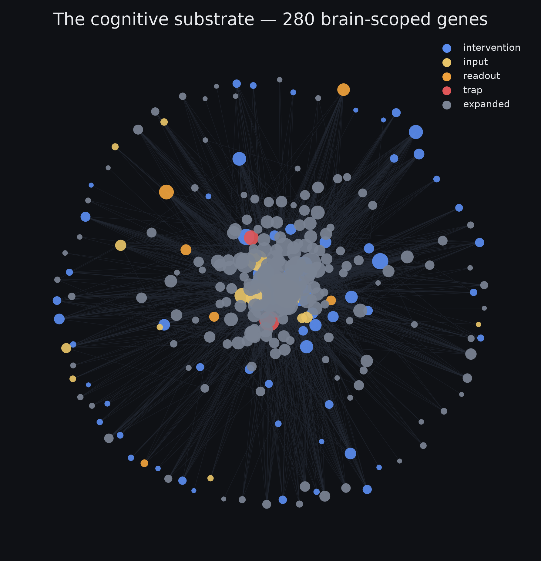
After pruning: 280 nodes in four layers — 70 intervention "knobs", 15 systemic inputs, 6 disease readouts, 2 off-limits, and 187 one-hop neighbors — with 3,912 directed edges (2,871 signed: 2,253 activating, 618 inhibiting) and a single 200-node feedback loop.
2. The propagation operator
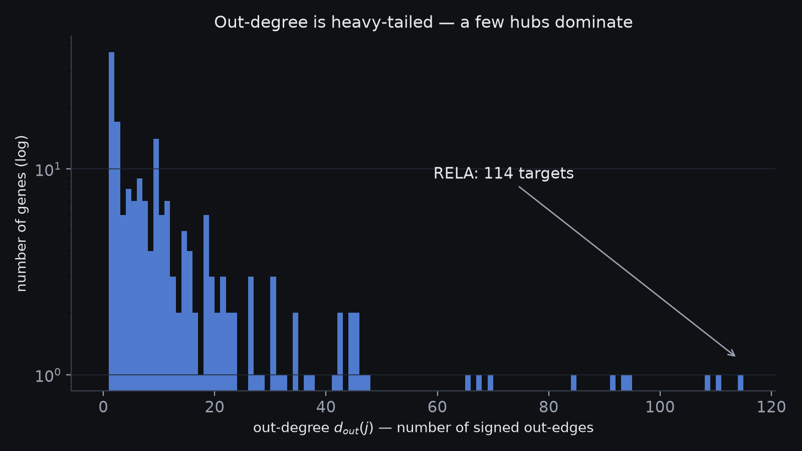
Put the edges in a matrix $W$: the entry $W_{ij}$ is $+1$, $-1$, or $0$ for the effect of gene $j$ on gene $i$ (oriented so $(Wx)_i$ is what flows into $i$). A hub gene with many out-edges would swamp everything, so I divide each gene's column by its out-degree — the same trick as Google's PageRank[3] ($d^{\mathrm{out}}_j=\sum_i|W_{ij}|$):
In words — spread each gene's outgoing effect evenly across the genes it points at, so one gene that talks to everyone can't dominate.
Each column now sums to 1 in absolute value, which forces the largest eigenvalue to be $\le 1$ (Perron–Frobenius) and keeps the next step stable (measured: $\rho(\hat W)=0.544$). Dividing by out-degree is the right move for a directed graph, where the problem is out-hubs; the symmetric GCN version $D^{-1/2}\tilde W D^{-1/2}$[6] is for undirected graphs.
3. Propagation by random-walk-with-restart
To see what a nudge does, push a signal $p$ into one gene and let it spread — but pull a fraction $\alpha$ back to the source at each step, so it stays near where it started[5],[4]:
In words — at each step, spread the signal one hop, but yank a fixed slice $\alpha$ of it back to the gene you started from.
Solving for the value it settles to gives a closed form (a sum over every path length $k$):
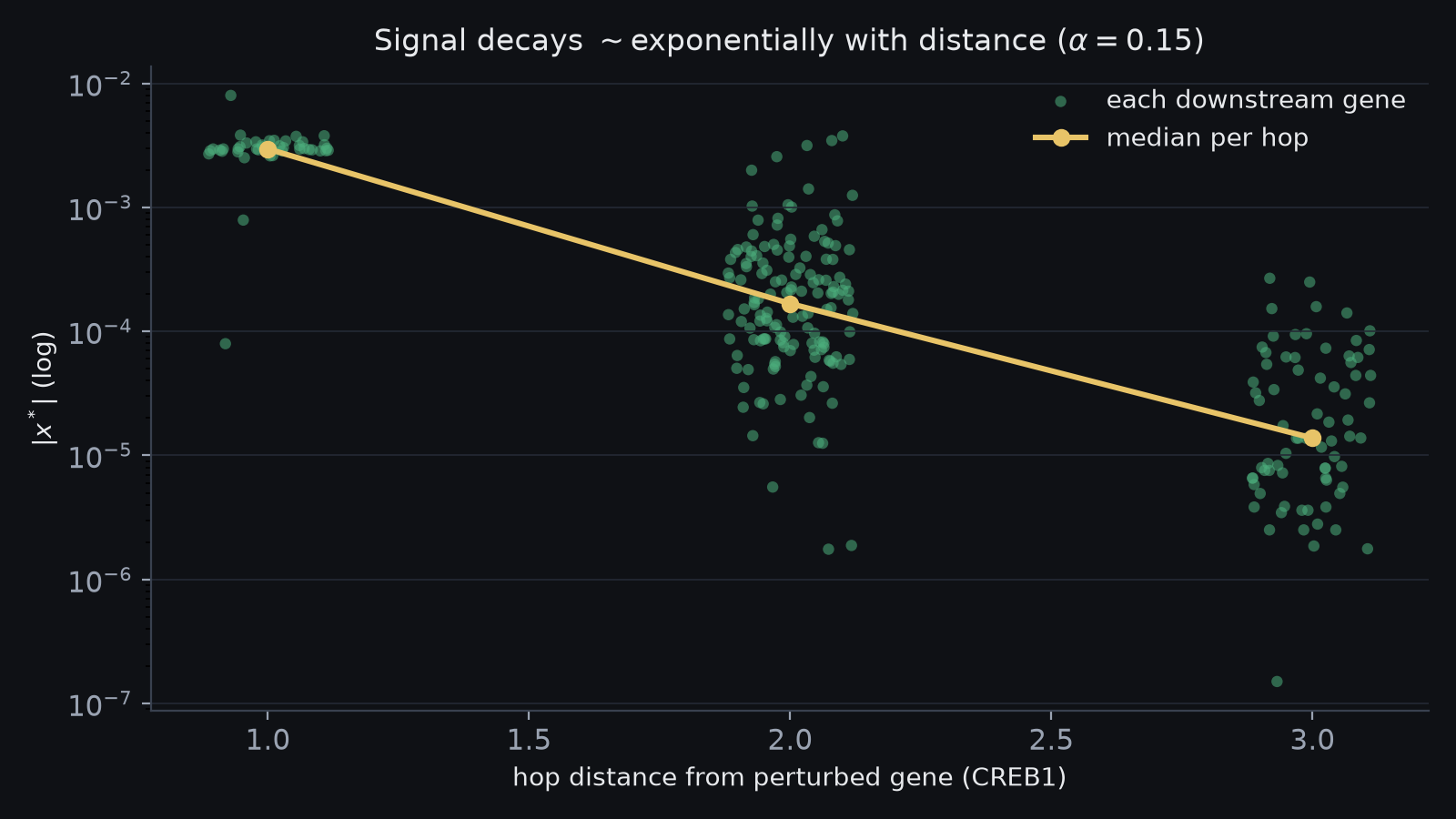
In words — the settled response; each extra hop is discounted by $(1-\alpha)^k$, so far-away genes barely feel it.
Because far hops are discounted, the effect stays local — most of the signal is gone within a few hops. The 200-node feedback loop is why we solve for a settled value instead of taking a single push.
4. Controllability
Can a few inputs steer the whole thing? Written as a linear system with input map $B$ (the genes we can drive), $\dot{x}=Wx+Bu$, it's fully steerable when the controllability matrix has full rank (Kalman[7]):
In words — you can reach any state exactly when your inputs, pushed through more and more hops, together cover all $N$ directions.
Testing that directly is impractical at this size, so I use structural controllability (Lin[8]; Liu–Slotine–Barabási[9]): the fewest genes you must control is the number left unmatched after pairing up the network as well as possible,
In words — match each gene to one it directly drives; whatever's left over is what you have to control by hand.
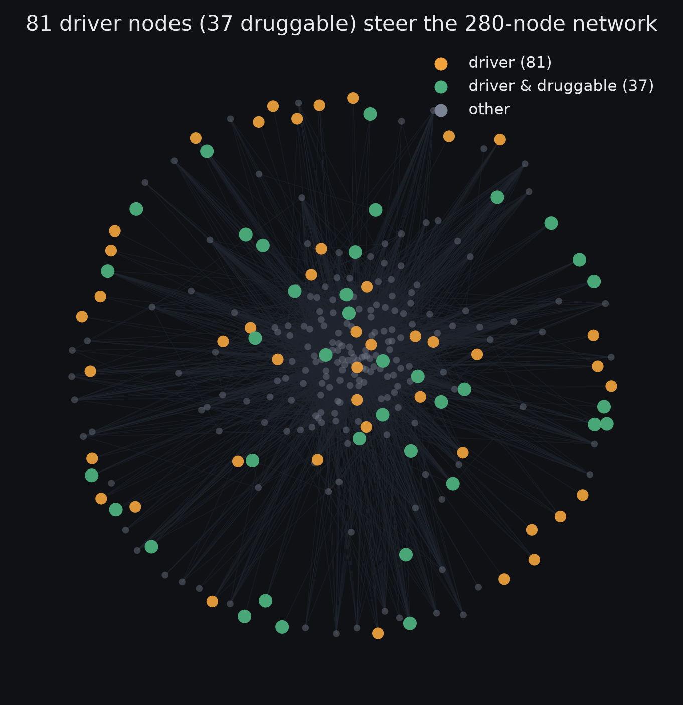
The matching is found with Hopcroft–Karp[10]. The result: all 280 genes are reachable, but full control would need 81 driver genes and only 37 of those are druggable — so you can't push it to any state you like. You can steer the readouts you actually care about (target control[11]), which takes fewer inputs, and that's the setting the optimizer works in.
| quantity | value |
|---|---|
| druggable inputs $|\mathcal D|$ | 172 |
| reachable $|R|/N$ | 280 / 280 |
| min drivers $N_D$ (full control) | 81 |
| drivers that are druggable | 37 / 81 |
| feedback component (SCC) | 200 |
Formal target controllability
"You can steer the readouts" was an assumption above. The actual test: with outputs $y=Cx$ selecting the scored targets $S$, that set is fully controllable iff the target-controllability matrix has full row rank[11]:
In words — count how many independent directions of the target state your inputs can actually reach. Fewer than $|S|$ means you can push it along a subspace, but not drive it anywhere you like.
Against the 78 scored targets present in the graph:
| input set | inputs | rank / |S| | coverage |
|---|---|---|---|
| constrained drivers (un-defended, §7) | 7 | 72 / 78 | 92% |
| all druggable knobs (unconstrained) | 24 | 73 / 78 | 94% |
| every node (graph ceiling) | 280 | 78 / 78 | 100% |
The seven un-defended drivers span 92% of the target space — they steer it rather than merely nudge it. And refusing to push the defended hubs costs just one dimension (92% vs 94%), so the constraint in §7 is nearly free. (Within the model, of course — the graph is the graph.)
5. Target state and objective
The target is a vector $d$ of desired changes. The key fact: most brain variables aren't "more is better" — they have a sweet spot, an inverted-U (Yerkes–Dodson[18]; Arnsten[19]): dopamine, arousal, cortisol, excitation/inhibition balance, mTOR. Benefit is how much closer to the target you get:
In words — positive if the nudge moved a gene toward its ideal level, negative if it pushed past it.
Total benefit weights each gene by how sure we are of its target (readouts count for nothing); cost is how hard you push plus how much you disturb genes outside the target set:
In words — add up the good across all genes, then subtract the cost: effort plus collateral movement elsewhere.
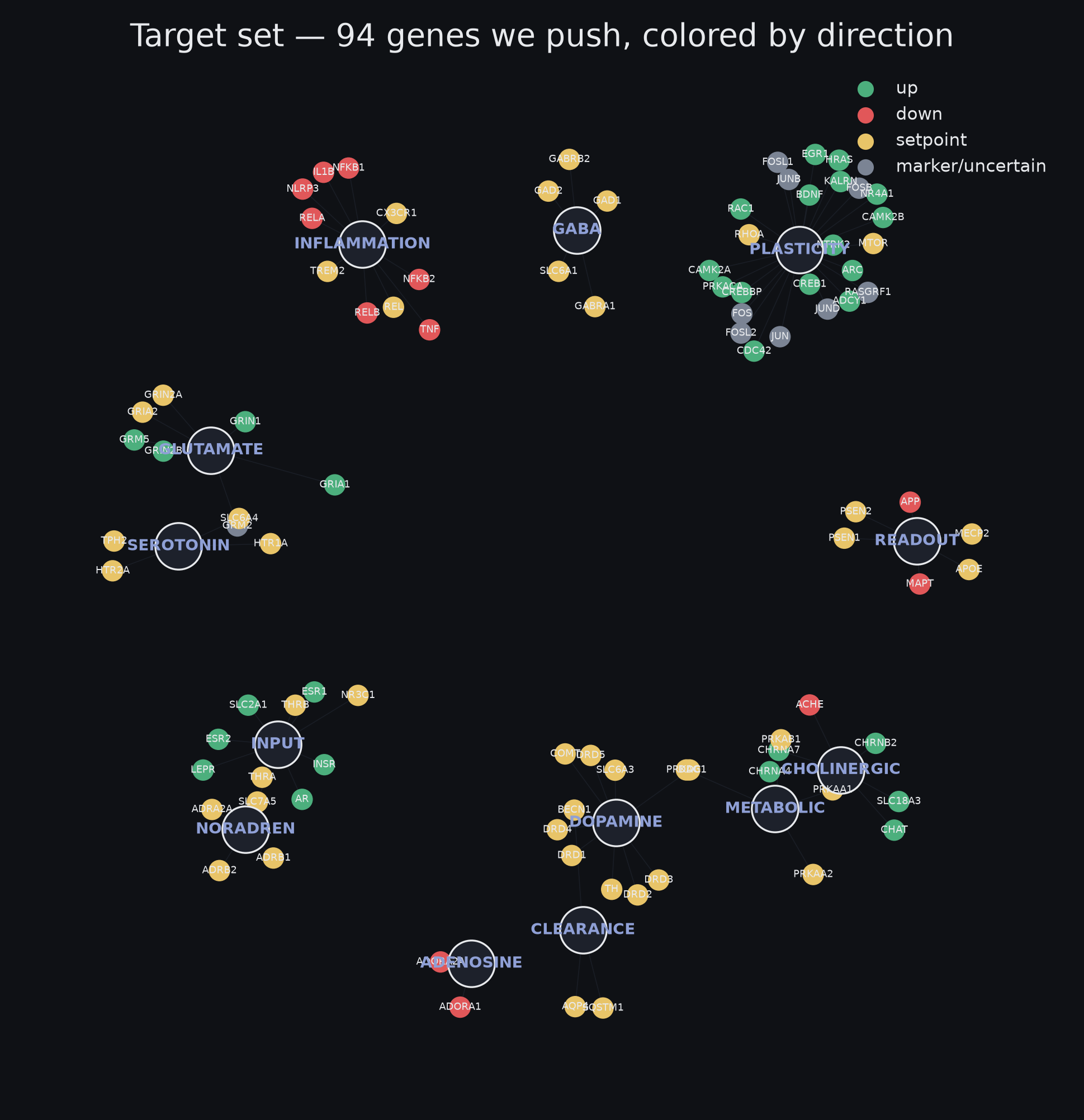
The current target vector covers 94 genes: 43 set-point, 30 up, 12 down.
6. Uncertainty quantification
Our confidence in each target isn't uniform — some directions are well-established, others shaky — so a single score would overstate precision. We run it many times, sampling each target's confidence weight within its interval (Monte-Carlo[12]), and report a range instead of a point,
In words — run it many times, sort the scores, and report the middle 90% as an honest range.
Then use Sobol indices[13],[14] to see which unknown is driving the range:
In words — of all the wobble in the score, how much comes from each unknown — so you know which fact to go check first.
Edge strengths are deliberately left out of this: they're treated as sign-only (unit weight), because there's no principled distribution to sample — inventing one would add noise, not information.
7. Optimization
There's no single best answer — more benefit usually costs more — so the output is a trade-off curve (a Pareto front). I trace it with the ε-constraint method[15]: get the most benefit while keeping cost under a cap $\varepsilon$, then slide the cap:
In words — squeeze out the most benefit at each cost budget, then vary the budget to draw the whole curve.
A plain weighted sum, $\max_p B(p)-\lambda C(p)$, would quietly skip part of the curve when it bends the wrong way (a non-convex front)[16],[17]; ε-constraint doesn't, and the small size makes it cheap to run.
A necessary constraint. The optimizer may only push un-defended upstream drivers — nodes that cascade (out-degree > 0) but aren't heavily regulated (low in-degree). Defended convergence hubs like BDNF and CREB1 are excluded from the push set: they have many regulators (BDNF has 15) that fight a direct push — homeostasis — so we treat them as targets we move indirectly, not levers we pull. (The Liu–Barabási driver set is non-unique, so we use the deterministic in-degree criterion instead.)
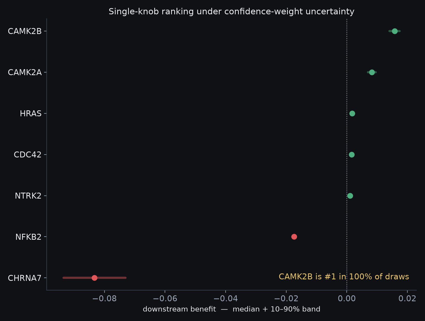
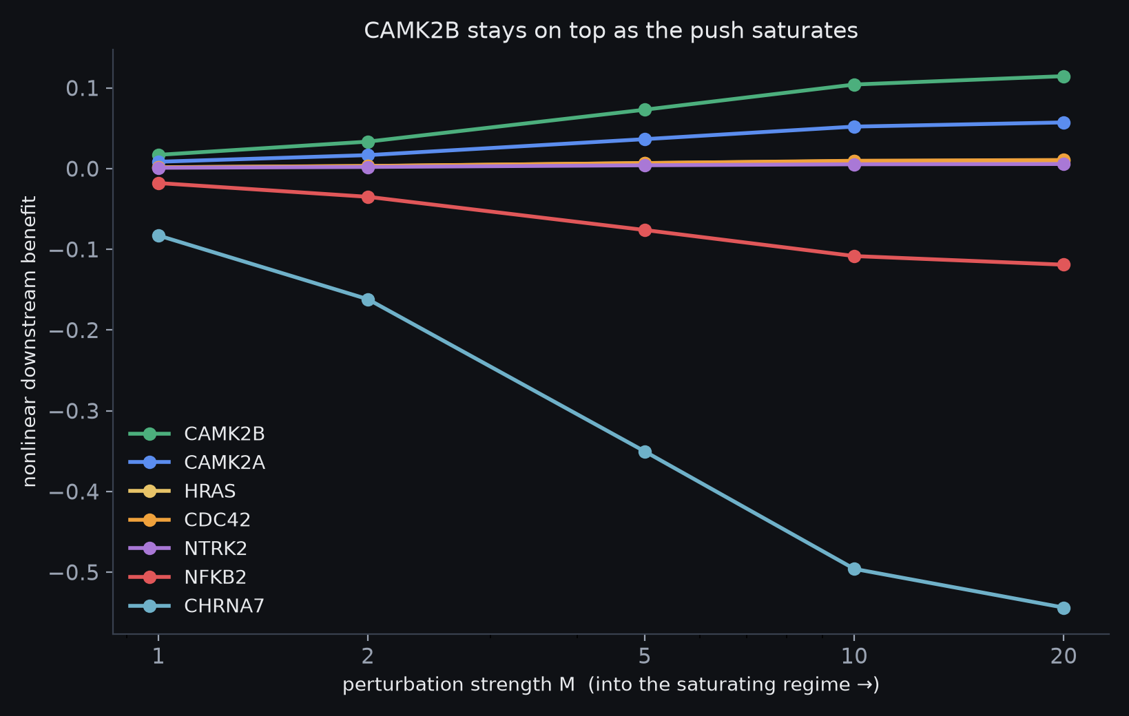
Result. Among the un-defended drivers, counting only the downstream effect (so a gene isn't credited for moving itself), CAMK2B (CaMKIIβ, in-degree 0) is the top single lever — #1 in 100% of the 2,000 uncertainty draws, and it holds #1 under the nonlinear cross-check (§8). The benefit is modest: un-defended drivers reach less of the network than the defended hubs we deliberately can't push — which is the honest, un-inflated answer.
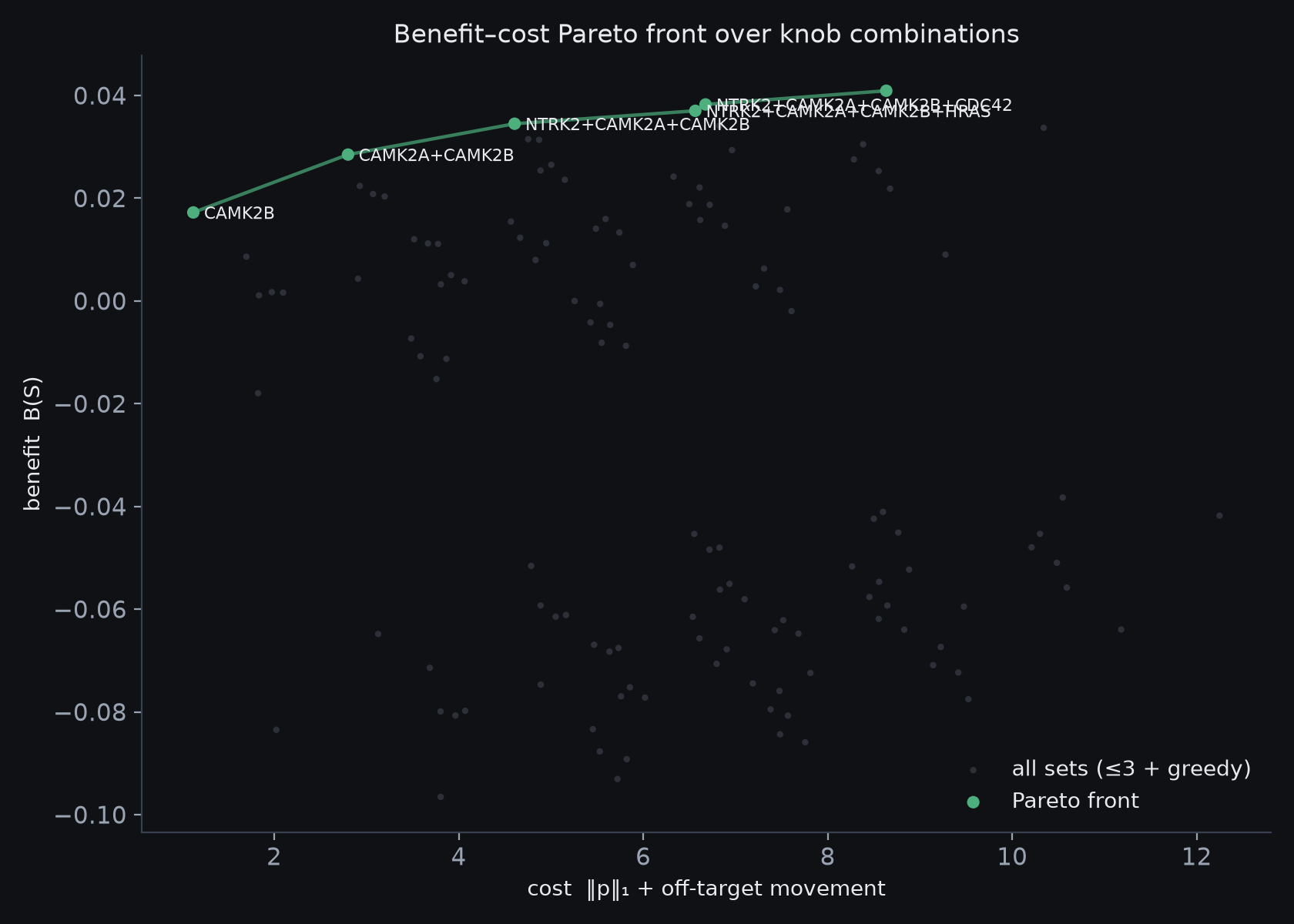
For combinations, the constrained set is small enough that no heuristic is needed: all $2^{7}-1=127$ subsets are evaluated exhaustively, so the front below is provably optimal within the constraint — not a greedy approximation that might have missed a better set. (Greedy forward selection is still run as a cross-check; it lands on the front but misses one point, which is the reason to prefer the exhaustive sweep while it stays cheap.)
| # | knob set | benefit | cost |
|---|---|---|---|
| 1 | CAMK2B | +0.0172 | 1.12 |
| 2 | CAMK2A + CAMK2B | +0.0285 | 2.80 |
| 3 | NTRK2 + CAMK2A + CAMK2B | +0.0345 | 4.61 |
| 4 | NTRK2 + CAMK2A + CAMK2B + HRAS | +0.0370 | 6.57 |
| 5 | NTRK2 + CAMK2A + CAMK2B + CDC42 | +0.0383 | 6.68 |
| 6 | NTRK2 + CAMK2A + CAMK2B + CDC42 + HRAS | +0.0409 | 8.64 |
The knee is CAMK2B alone — best benefit per unit cost — followed by steep diminishing returns: the last four points buy roughly twice the benefit for roughly eight times the cost. The drivers act on largely independent downstream, so combinations are close to additive (no synergistic stack), and the efficient set stays small.
8. Validation
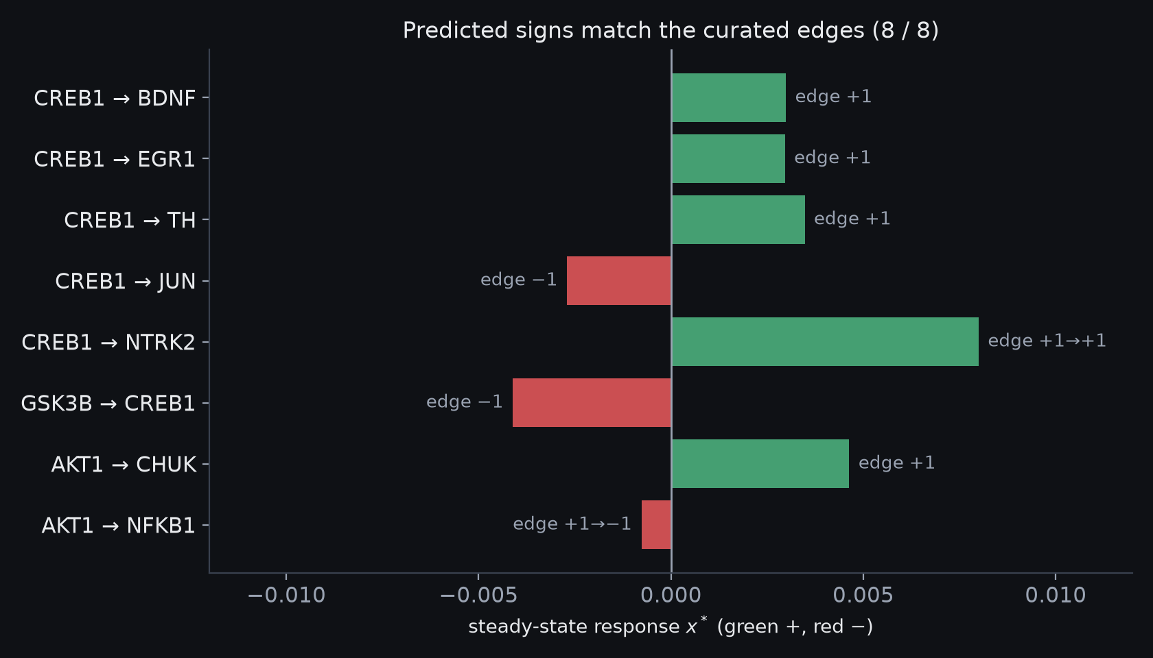
The engine is test-driven throughout — each stage is gated by unit tests (sign propagation, the resolvent, the objective, the confidence bands, the Pareto front, and the nonlinear map). The main sign check: push one gene by $+1$ and confirm the response sign matches the edge sign in the database — not the model. All eight match ($\alpha=0.15$, $\rho(\hat W)=0.544$).
| perturb | → target | edge | $x^{*}$ | check |
|---|---|---|---|---|
| CREB1 ↑ | BDNF | +1 | +0.0030 | ✓ |
| CREB1 ↑ | JUN | −1 | −0.0027 | ✓ flip |
| CREB1 ↑ | NTRK2 | +1→+1 | +0.0080 | ✓ net |
| GSK3B ↑ | CREB1 | −1 | −0.0041 | ✓ inhib |
| AKT1 ↑ | NFKB1 | +1→−1 | −0.0008 | ✓ net-flip |
One nice check on the operator: two-hop NTRK2 moves more than one-hop BDNF, because
CREB1's ~40 out-edges split its signal while BDNF's single out-edge passes it straight through — exactly what
equation (2) predicts.
Nonlinear cross-check
The whole engine is linear, so the headline (§7) could be an artifact of that. We re-ran the constrained ranking under a saturating (tanh) propagation and pushed knobs progressively harder into the nonlinear regime, where the linear approximation is meant to break. CAMK2B stays #1 at every strength — its lead widens as the system saturates — and combinations stay roughly additive, so no synergy appears. The finding survives.
9. Groundedness and assumptions
The layers rest on very different evidence: brain-scoping is computed, edge signs are curated from causal databases, edge strengths are mostly sign-only, and the target vector is hand-built by me. $\hat W$ is a linear (first-order) stand-in for nonlinear biology, so results hold for small nudges near the resting state, not big ones. Everything above is internally consistent and tested; none of it is externally validated.
Concretely, the result "CAMK2B is the best lever" is a statement about this graph under this objective. For it to mean anything about an actual brain, all of the following would have to hold — and I have checked none of them:
- the edge set is roughly complete for this subsystem (it isn't — the graph is sparse, and absent edges are indistinguishable from absent biology)
- sign-only weights are a fair stand-in for real interaction strengths
- the hand-built target vector actually describes a learning-optimal state, rather than my reading of it
- a "push" on a gene corresponds to something a real intervention does — dose, timing, tissue, and compensation are all outside the model
- nothing important is missing that isn't a gene: metabolism, circuit dynamics, glia, and everything downstream of transcription
So the honest output is an ordered list under stated assumptions and a trade-off map — not fold-changes, not predictions, and emphatically not medical advice. The value of the exercise is the machinery, not the answer: a working pipeline from public graph to constrained, uncertainty-quantified, provably-optimal-within-the-constraint intervention sets. Point it at a better graph and a validated target vector and the same code would be worth something. As it stands it's a math experiment that happens to be about neurons.
10. Status & roadmap
Built, tested, and run: the full pipeline — substrate (§1), operator and RWR engine (§2–3), structural and formal target controllability (§4), the set-point objective (§5), the uncertainty pass (§6), the constrained ε-constraint optimizer over an exhaustive combination sweep (§7), and the nonlinear cross-check (§8). Further out: fitting real edge strengths where measured data exists, a richer intervention model (dose, timing), and validation against real perturbation datasets — the last of which is the only thing that would turn any of this from an exercise into evidence. This is a living write-up; it will change as those pieces land.
References
- Chandak, P., Huang, K., Zitnik, M. Building a knowledge graph to enable precision medicine. Scientific Data 10, 67 (2023).
- Himmelstein, D.S. et al. Systematic integration of biomedical knowledge prioritizes drugs for repurposing. eLife 6, e26726 (2017).
- Page, L., Brin, S., Motwani, R., Winograd, T. The PageRank Citation Ranking: Bringing Order to the Web. Stanford InfoLab (1999).
- Gasteiger, J., Bojchevski, A., Günnemann, S. Predict then Propagate: Graph Neural Networks meet Personalized PageRank. ICLR (2019).
- Tong, H., Faloutsos, C., Pan, J-Y. Fast Random Walk with Restart and Its Applications. ICDM (2006).
- Kipf, T.N., Welling, M. Semi-Supervised Classification with Graph Convolutional Networks. ICLR (2017).
- Kalman, R.E. Mathematical Description of Linear Dynamical Systems. J. SIAM Control 1(2), 152–192 (1963).
- Lin, C-T. Structural Controllability. IEEE Trans. Automatic Control 19(3), 201–208 (1974).
- Liu, Y-Y., Slotine, J-J., Barabási, A-L. Controllability of complex networks. Nature 473, 167–173 (2011).
- Hopcroft, J.E., Karp, R.M. An $n^{5/2}$ Algorithm for Maximum Matchings in Bipartite Graphs. SIAM J. Comput. 2(4), 225–231 (1973).
- Gao, J., Liu, Y-Y., D'Souza, R.M., Barabási, A-L. Target control of complex networks. Nature Communications 5, 5415 (2014).
- JCGM 101:2008. Evaluation of measurement data — Supplement 1 to the GUM — Propagation of distributions using a Monte Carlo method. BIPM (2008).
- Sobol, I.M. Global sensitivity indices for nonlinear mathematical models and their Monte Carlo estimates. Math. Comput. Simul. 55, 271–280 (2001).
- Saltelli, A. et al. Global Sensitivity Analysis: The Primer. Wiley (2008).
- Haimes, Y.Y., Lasdon, L.S., Wismer, D.A. On a bicriterion formulation … the ε-constraint method. IEEE Trans. Syst. Man Cybern. 1(3), 296–297 (1971).
- Boyd, S., Vandenberghe, L. Convex Optimization (§4.7, scalarization & Pareto optimality). Cambridge Univ. Press (2004).
- Marler, R.T., Arora, J.S. Survey of multi-objective optimization methods for engineering. Struct. Multidiscip. Optim. 26, 369–395 (2004).
- Yerkes, R.M., Dodson, J.D. The relation of strength of stimulus to rapidity of habit-formation. J. Comp. Neurol. Psychol. 18, 459–482 (1908).
- Arnsten, A.F.T. Stress signalling pathways that impair prefrontal cortex structure and function. Nat. Rev. Neurosci. 10, 410–422 (2009).
Project overview · source code · versions: current · v1 (Jul 2026) · a personal learning project — not medical advice.